Algorithm Review
Algorithm review of M.H.Alsuwaiyel, Algorithms design techniques and Analysis, Publishing House of Electronics Industry.
分析 Algorithmic Analysis
Binary Search
1 | low←1; high←n; j←0; |
The number of comparisons performed by the algorithm Binary Search on a sorted array of size n is at most $\lfloor log n \rfloor+1$
Merging Two Sorted Lists
1 | s←p; t←q+1; k←p; |
此处需要分析
Selection Sort
1 | for i←1 to n-1 |
Insertion Sort
1 | for i←2 to n |
Bottom-Up Merge Sorting
1 | t←1; |
递归 Techniques Based on Recursion
归纳 induction
Given a problem with parameter n, designing an algorithm by induction is based on the fact that if we know how to solve the problem when presented with a parameter less than n, called the induction hypothesis, then our task reduces to extending that solution to include those instances with parameter n.
Radix Sort
Let $L=\{a_1, a_2, …, a_n\}$ be a list of n numbers each consisting of exactly $k$ digits. That is, each number is of the form $d_kd_{k-1}…d_1$, where each $d_i$ is a digit between 0 and 9.
In this problem, instead of applying induction on n, the number of objects, we use induction on k, the size of each integer.
If the numbers are first distributed into the lists by their least significant digit, then a very efficient algorithm results.
Suppose that the numbers are sorted lexicographically according to their least k-1 digits, i.e., digits $d_{k-1}, d_{k-2}, …, d_1$.
After sorting them on their kth digits, they will eventually be sorted.
First, distribute the numbers into 10 lists $L_0, L_1, …, L_9$ according to digit $d_1$ so that those numbers with $d_1=0$ constitute list $L_0$, those with $d_1=1$ constitute list $L_1$ and so on.
Next, the lists are coalesced in the order $L_0, L_1, …, L_9$.
Then, they are distributed into 10 lists according to digit $d_2$, coalesced in order, and so on.
After distributing them according to $d_k$ and collecting them in order, all numbers will be sorted.
Example: Sort A nondecreasingly. A[1…5]=7467,3275,6792,9134,1239
Input: A linked list of numbers $L={a_1, a_2, …, a_n}$ and k, the number of digits.
Output: L sorted in nondecreasing order.1
2
3
4
5
6
7
8
9
10
11
12
13
14for j←1 to k
Prepare 10 empty lists L0, L1, …, L9;
while L is not empty
a←next element in L;
Delete a from L;
i←jth digit in a;
Append a to list Li;
end while;
L ←L0;
for i ←1 to 9
L←L, Li //Append list Li to L
end for;
end for;
return L;
Time Complexity: $\Theta(n)$
Space Complexity: $\Theta(n)$
Generating permutations
Generating all permutations of the numbers 1, 2, …, n.
Based on the assumption that if we can generate all the permutations of n-1 numbers, then we can get algorithms for generating all the permutations of n numbers.
Generate all the permutations of the numbers 2, 3, …, n and add the number 1 to the beginning of each permutation.
Generate all permutations of the numbers 1, 3, 4, …, n and add the number 2 to the beginning of each permutation.
Repeat this procedure until finally the permutations of 1, 2, …, n-1 are generated and the number n is added at the beginning of each permutation.
Input: A positive integer n;
Output: All permutations of the numbers 1, 2, …, n;
1 | for j←1 to n |
Time Complexity: $\Theta(nn!)$
Space Complexity: $\Theta(n)$
Find Majority
Let A[1…n] be a sequence of integers. An integer a in A is called the majority if it appears more than $\lfloor n/2 \rfloor$ times in A.
For example:
Sequence 1, 3, 2, 3, 3, 4, 3: 3 is the majority element since 3 appears 4 times which is more than $\lfloor n/2 \rfloor$
Sequence 1, 3, 2, 3, 3, 4: 3 is not the majority element since 3 appears three times which is equal to $\lfloor n/2 \rfloor$, but not more than $\lfloor n/2 \rfloor$
If two different elements in the original sequence are removed, then the majority in the original sequence remains the majority in the new sequence.
The above observation suggests the following procedure for finding an element that is candidate for being the majority.
Let x=A[1] and set a counter to 1.
Starting from A[2], scan the elements one by one increasing the counter by one if the current element is equal to x and decreasing the counter by one if the current element is not equal to x.
If all the elements have been scanned and the counter is greater than zero, then return x as the candidate.
If the counter becomes 0 when comparing x with A[j], 1< j < n, then call procedure candidate recursively on the elements A[j+1…n].
Input: An array A[1…n] of n elements;
Output: The majority element if it exists; otherwise none;1
2
3
4
5
6
7
8
9
10
11
12
13
14
15
16
17 x←candidate(1);
count←0;
for j←1 to n
if A[j]=x then count←count+1;
end for;
if count> [n/2] then return x;
else return none;
candidate(m)
j←m; x←A[m]; count←1;
while j<n and count>0
j ←j+1;
if A[j]=x then count ←count+1;
else count ←count-1;
end while;
if j=n then return x;
else return candidate(j+1);
分而治之 Divide and Conquer
A divide-and-conquer algorithm divides the problem instance into a number of subinstances (in most cases 2), recursively solves each subinsance separately, and then combines the solutions to the subinstances to obtain the solution to the original problem instance.
The Divide and Conquer Paradigm
The divide step: the input is partitioned into $p\geq1$ parts, each of size strictly less than n.
The conquer step: performing p recursive call(s) if the problem size is greater than some predefined threshold n0.
The combine step: the solutions to the p recursive call(s) are combined to obtain the desired output.
- If the size of the instance I is “small”, then solve the problem using a straightforward method and return the answer. Otherwise, continue to the next step;
- Divide the instance I into p subinstances I1, I2, …, Ip of approximately the same size;
- Recursively call the algorithm on each subinstance Ij, $1\leq j\leq p$, to obtain p partial solutions;
- Combine the results of the p partial solutions to obtain the solution to the original instance I. Return the solution of instance I.
Finding kth Smallest Element
The media of a sequence of n sorted numbers A[1…n] is the “middle” element.
If n is odd, then the middle element is the (n+1)/2th element in the sequence.
If n is even, then there are two middle elements occurring at positions n/2 and n/2+1. In this case, we will choose the n/2th smallest element.
Thus, in both cases, the median is the $\lceil n/2 \rceil$th smallest element.
The kth smallest element is a general case.
Input: An array A[1…n] of n elements and an integer k, $1\leq k\leq n$;
Output: The kth smallest element in A;
select(A, 1, n, k);
1 | select(A, low, high, k) |
The kth smallest element in a set of n elements drawn from a linearly ordered set can be found in $\Theta(n)$ time.
Quicksort
Let A[low…high] be an array of n numbers, and x=A[low].
We consider the problem of rearranging the elements in A so that all elements less than or equal to x precede x which in turn precedes all elements greater than x.
After permuting the element in the array, x will be A[w] for some w, low<=w<=high. The action of rearrangement is also called splitting or partitioning around x, which is called the pivot or splitting element.
We say that an element A[j] is in its proper position or correct position if it is neither smaller than the elements in A[low…j-1] nor larger than the elements in A[j+1…high].
After partitioning an array A using $x\in A$ as a pivot, x will be in its correct position.
Input: An array of elements A[low…high];
Output: A with its elements rearranged, if necessary; w, the new position of the splitting element A[low];1
2
3
4
5
6
7
8
9
10
11
12split(A[...], w)
i←low;
x←A[low];
for j←low+1 to high
if A[j]<=x then
i←i+1;
if i≠j then interchange A[i] and A[j];
end if;
end for;
interchange A[low] and A[i];
w←i;
return A and w;
The number of element comparisons performed by Algorithm SPLIT is exactly n-1. Thus, its time complexity is $\Theta(n)$.
The only extra space used is that needed to hold its local variables. Therefore, the space complexity is $\Theta(1)$.
Input: An array A[1…n] of n elements;
Output: The elements in A sorted in nondecreasing order;
quicksort(A, 1, n);1
2
3
4
5
6quicksort(A, low, high)
if low<high then
SPLIT(A[low…high], w) //w is the new position of A[low];
quicksort(A, low, w-1);
quicksort(A, w+1, high);
end if;
The average number of comparisons performed by Algorithm QUICKSORT to sort an array of n elements is $\Theta(nlogn)$.
动态规划 Dynamic Programming
An algorithm that employs the dynamic programming technique is not recursive by itself, but the underlying solution of the problem is usually stated in the form of a recursive function.
This technique resorts to evaluating the recurrence in a bottom-up manner, saving intermediate results that are used later on to compute the desired solution.
This technique applies to many combinatorial optimization problems to derive efficient algorithms.
Longest Common Subsequence
Given two strings A and B of lengths n and m, respectively, over an alphabet $\sum$, determine the length of the longest subsequence that is common to both A and B.
A subsequence of $A=a_1a_2…a_n$ is a string of the form $a_{i1}a_{i2}…a_{ik}$, where each $i_j$ is between 1 and n and $1\leq i_1<i_2<…<i_k\leq n$.
Let $A=a_1a_2…a_n$ and $B=b_1b_2…b_m$.
Let L[i, j] denote the length of a longest common subsequence of $a_1a_2…a_i$ and $b_1b_2…b_j$. $0\leq i\leq n, 0\leq j\leq m$. When i or j be 0, it means the corresponding string is empty.
Naturally, if i=0 or j=0; the L[i, j]=0
Suppose that both i and j are greater than 0. Then
If $a_i=b_j,L[i,j]=L[i-1,j-1]+1$
If $a_i\ne b_j,L[i,j]=max\{L[i,j-1],L[i-1,j]\}$
We get the following recurrence for computing the length of the longest common subsequence of A and B:
We use an $(n+1)\times(m+1)$ table to compute the values of $L[i, j]$ for each pair of values of i and j, $0\leq i\leq n, 0\leq j\leq m$.
We only need to fill the table $L[0…n, 0…m]$ row by row using the previous formula.
Example: A=zxyxyz, B=xyyzx
Input: Two strings A and B of lengths n and m, respectively, over an alphabet $\sum$;
Output: The length of the longest common subsequence of A and B.1
2
3
4
5
6
7
8
9
10
11
12
13
14for i←0 to n
L[i, 0]←0;
end for;
for j←0 to m
L[0, j]←0;
end for;
for i←1 to n
for j←1 to m
if ai=bj then L[i, j]←L[i-1, j-1]+1;
else L[i, j]←max{L[i, j-1], L[i-1, j]};
end if;
end for;
end for;
return L[n, m];
Time Complexity: $\Theta(nm)$
Space Complexity: $\Theta(\min\{n,m\})$
The Dynamic Programming Paradigm
The idea of saving solutions to subproblems in order to avoid their recomputation is the basis of this powerful method.
This is usually the case in many combinatorial optimization problems in which the solution can be expressed in the form of a recurrence whose direct solution causes subinstances to be computed more than once.
An important observation about the working of dynamic programming is that the algorithm computes an optimal solution to every subinstance of the original instance considered by the algorithm.
This argument illustrates an important principle in algorithm design called the principle of optimality: Given an optimal sequence of decisions, each subsequence must be an optimal sequence of decisions by itself.
All-Pairs Shortest Path
$d_{i,j}^0=l[i,j]$
$d_{i,j}^1$ is the length of a shortest path from i to j that does not pass through any vertex except possibly vertex 1
$d_{i,j}^2$ is the length of a shortest path from i to j that does not pass through any vertex except possibly vertex 1 or vertex 2 or both
$d_{i,j}^n$ is the length of a shortest path from i to j, i.e. the distance from i to j
We can compute $d_{i,j}^k$ recursively as follows:
Here,We use Floyd Algorithm !
use n+1 matrices $D_0, D_1, D_2, …, D_n$ of dimension $n\times n$ to compute the lengths of the shortest constrained paths.
Initially, we set $D_0[i, i]=0, D_0[i, j]=l[i, j] if\ i\ne j$ and (i, j) is an edge in G; otherwise $D_0[i, j]=\infty $.
We then make n iterations such that after the kth iteration, $D_k[i, j]$ contains the value of a shortest length path from vertex i to vertex j that does not pass through any vertex numbered higher than k.
Thus, in the kth iteration, we compute $D_k[i, j]$ using the formula
Example:
Input: An $n\times n$ matrix $l[1…n, 1…n]$ such that $l[i, j]$ is the length of the edge(i, j) in a directed graph G=({1, 2, …, n}, E);
Output: A matrix D with D[i, j]=the distance from i to j1
2
3
4
5
6
7
8D←l;
for k←1 to n
for i←1 to n
for j←1 to n
D[i, j]=min{D[i, j], D[i, k]+D[k, j]);
end for;
end for;
end for;
Time Complexity: $\Theta(n^3)$
Space Complexity: $\Theta(n^2)$
Knapsack Problem
Let $U={u_1, u_2, …, u_n}$ be a set of n items to be packed in a knapsack of size C. for $1\leq j\leq n$, let $s_j$ and $v_j$ be the size and value of the jth item, respectively, where C and sj, vj, 1jn, are all positive integers.
The objective is to fill the knapsack with some items for U whose total size is at most C and such that their total value is maximum. Assume without loss of generality that the size of each item does not exceed C.
More formally, given U of n items, we want to find a subset $S\in U$ such that
is maximized subject to the constraint
This version of the knapsack problem is sometimes referred to in the literature as the 0/1 knapsack problem. This is because the knapsack cannot contain more than one item of the same type.
Let V[i, j] denote the value obtained by filling a knapsack of size j with items taken from the first i items {u1, u2, …, ui} in an optimal way. Here the range of i is from 0 to n and the range of j is from 0 to C. Thus, what we seek is the value V[n, C].
Obviously, V[0, j] is 0 for all values of j, as there is nothing in the knapsack. On the other hand, V[i, 0] is 0 for all values of i since nothing can be put in a knapsack of size 0.
V[i, j], where i>0 and j>0, is the maximum of the following two quantities:
V[i-1, j]: The maximum value obtained by filling a knapsack of size j with items taken from $\{u_1, u_2, …, u_{i-1}\}$ only in an optimal way.
$V[i-1, j-s_i]+v_i$: The maximum value obtained by filling a knapsack of size $j-s_i$ with items taken from $\{u_1, u_2, …, u_{i-1}\}$ in an optimal way plus the value of item $u_i$. This case applies only if $j\geq s_i$ and it amounts to adding item $u_i$ to the knapsack.
Then, we got the following recurrence for finding the value in an optimal packing:
Using dynamic programming to solve this integer programming problem is now straightforward. We use an $(n+1)\times (C+1)$ table to evaluate the values of V[i, j]. We only need to fill the table V[0…n, 0…C] row by row using the above formula.
Example:
C=9
U={u1, u2, u3, u4}
Si=2, 3, 4, 5
Vi=3, 4, 5, 7
Input: A set of items $U={u_1, u_2, …, u_n}$ with sizes $s_1, s_2, …, s_n$ and values $v_1, v_2, …, v_n$ and a knapsack capacity C.
Output: The maximum value of the function $\sum_{u_i\in S}v_i$ subject to $\sum_{u_i\in S}S_i\leq C$ for some subset of items $S\in U$.1
2
3
4
5
6
7
8
9
10
11
12
13for i←0 to n
V[i, 0]←0;
end for;
for j←0 to C
V[0, j]←0;
end for;
for i←1 to n
for j←1 to C
V[i, j]←V[i-1, j];
if si<=j then V[i, j] ← max{V[i, j], V[i-1, j-si]+vi};
end for;
end for;
return V[n, C];
Time Complexity: $\Theta(nC)$
Space Complexity: $\Theta(C)$
贪心 The Greedy Approach
As in the case of dynamic programming algorithms, greedy algorithms are usually designed to solve optimization problems in which a quantity is to be minimized or maximized.
Unlike dynamic programming algorithms, greedy algorithms typically consist of a n iterative procedure that tries to find a local optimal solution.
In some instances, these local optimal solutions translate to global optimal solutions. In others, they fail to give optimal solutions.
A greedy algorithm makes a correct guess on the basis of little calculation without worrying about the future. Thus, it builds a solution step by step. Each step increases the size of the partial solution and is based on local optimization.
The choice make is that which produces the largest immediate gain while maintaining feasibility.
Since each step consists of little work based on a small amount of information, the resulting algorithms are typically efficient.
The Fractional Knapsack Problem
Given n items of sizes s1, s2, …, sn, and values v1, v2, …, vn and size C, the knapsack capacity, the objective is to find nonnegative real numbers x1, x2, …, xn that maximize the sum
subject to the constraint
This problem can easily be solved using the following greedy strategy:
For each item compute yi=vi/si, the ratio of its value to its size.
Sort the items by decreasing ratio, and fill the knapsack with as much as possible from the first item, then the second, and so forth.
This problem reveals many of the characteristics of a greedy algorithm discussed above: The algorithm consists of a simple iterative procedure that selects that item which produces that largest immediate gain while maintaining feasibility.
Shortest Path Problem
Let G=(V, E) be a directed graph in which each edge has a nonnegative length, and a distinguished vertex s called the source. The single-source shortest path problem, or simply the shortest path problem, is to determine the distance from s to every other vertex in V, where the distance from vertex s to vertex x is defined as the length of a shortest path from s to x.
For simplicity, we will assume that V={1, 2, …, n} and s=1.
This problem can be solved using a greedy technique known as Dijkstra algorithm.
The set of vertices is partitioned into two sets X and Y so that X is the set of vertices whose distance from the source has already been determined, while Y contains the rest vertices. Thus, initially X={1} and Y={2, 3, …, n}.
Associated with each vertex y in Y is a label $\lambda[y]$, which is the length of a shortest path that passes only through vertices in X. Thus, initially
At each step, we select a vertex $y\in Y$ with minimum $\lambda$ and move it to X, and $\lambda$ of each vertex $w\in Y$ that is adjacent to y is updated indicating that a shorter path to w via y has been discovered.
The above process is repeated until Y is empty.
Finally, $lambda$ of each vertex in X is the distance from the source vertex to this one.
Example: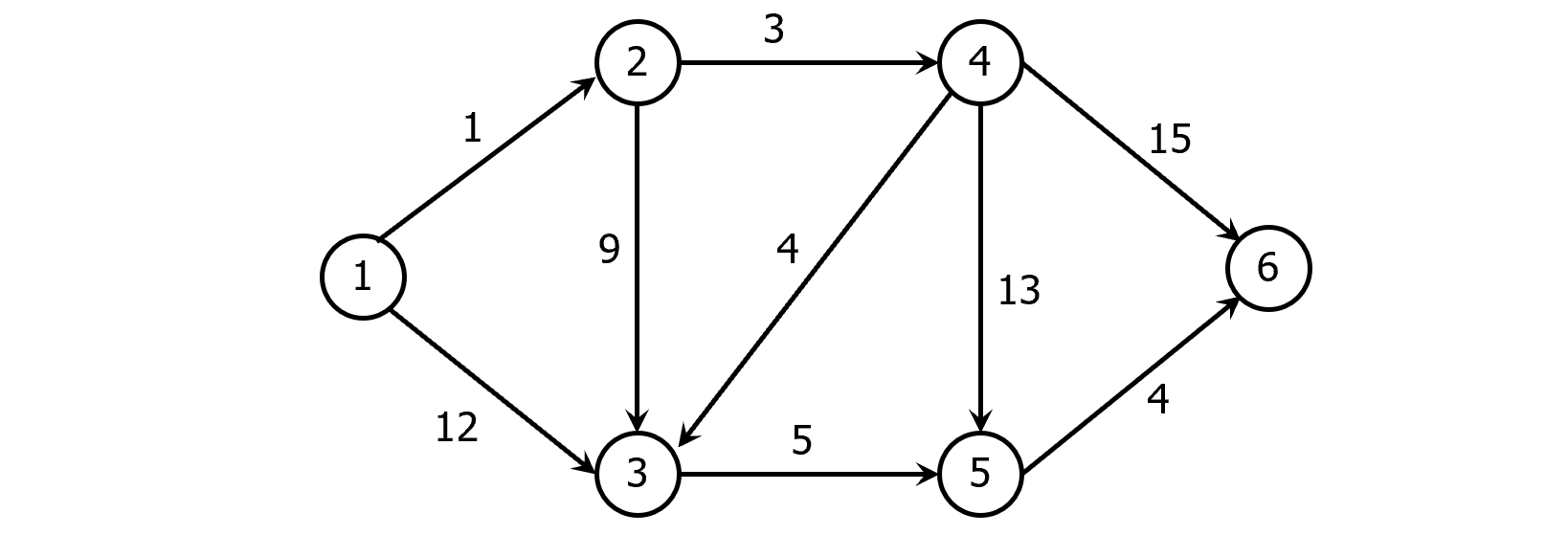
Input: A weighted directed graph G=(V, E), where V={1, 2, …, n};
Output: The distance from vertex 1 to every other vertex in G;1
2
3
4
5
6
7
8
9
10
11
12
13
14
15X={1}; Y←V-{1}; λ[1]←0;
for y←2 to n
if y is adjacent to 1 then λ[y]←length[1, y];
else λ[y]← ∞;
end if;
end for;
for j←1 to n-1
Let y∈Y be such that λ[y] is minimum;
X←X∪{y}; // add vertex y to X
Y←Y-{y}; // delete vertex y from Y
for each edge (y, w)
if w∈Y and λ[y]+length[y, w]<λ[w] then
λ[w]←λ[y]+length[y, w];
end for;
end for;
Given a directed graph G with nonnegative weights on its edges and a source vertex s, Algorithm DIJKSTRA finds the length of the distance from s to every other vertex in $\Theta(n^2)$ time.
MST / Minimum Cost Spanning Trees (Kruskal / Prim)
Let G=(V, E) be a connected undirected graph with weights on its edges.
A spanning tree (V, T) of G is a subgraph of G that is a tree.
If G is weighted and the sum of the weights of the edges in T is minimum, then (V, T) is called a minimum cost spanning tree or simply a minimum spanning tree.
Kruskal’s algorithm works by maintaining a forest consisting of several spanning trees that are gradually merged until finally the forest consists of exactly one tree.
The algorithm starts by sorting the edges in nondecreasing order by weight.
Next, starting from the forest (V, T) consisting of the vertices of the graph and none of its edges, the following step is repeated until (V, T) is transformed into a tree: Let (V, T) be the forest constructed so far, and let $e\in E-T$ be the current edge being considered. If adding e to T does not create a cycle, then include e in T; otherwise discard e.
This process will terminate after adding exactly n-1 edges.
Example: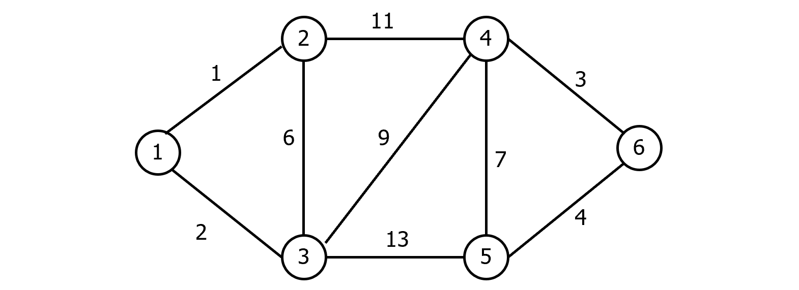
Huffman / File Compression
Suppose we are given a file, which is a string of characters. We wish to compress the file as much as possible in such a way that the original file can easily be reconstructed.
Let the set of characters in the file be C={c1, c2, …, cn}. Let also f(ci), $1\leq i \leq n$, be the frequency of character ci in the file, i.e., the number of times ci appears in the file.
Using a fixed number of bits to represent each character, called the encoding of the character, the size of the file depends only on the number of characters in the file.
Since the frequency of some characters may be much larger than others, it is reasonable to use variable length encodings.
Intuitively, those characters with large frequencies should be assigned short encodings, whereas long encodings may be assigned to those characters with small frequencies.
When the encodings vary in length, we stipulate that the encoding of one character must not be the prefix of the encoding of another character; such codes are called prefix codes.
For instance, if we assign the encodings 10 and 101 to the letters “a” and “b”, there will be an ambiguity as to whether 10 is the encoding of “a” or is the prefix of the encoding of the letter “b”.
Once the prefix constraint is satisfied, the decoding becomes unambiguous; the sequence of bits is scanned until an encoding of some character is found.
One way to “parse” a given sequence of bits is to use a full binary tree, in which each internal node has exactly two branches labeled by 0 an 1. The leaves in this tree corresponding to the characters. Each sequence of 0’s and 1’s on a path from the root to a leaf corresponds to a character encoding.
The algorithm presented is due to Huffman.
The algorithm consists of repeating the following procedure until C consists of only one character.
Let ci and cj be two characters with minimum frequencies.
Create a new node c whose frequency is the sum of the frequencies of ci and cj, and make ci and cj the children of c.
Let C=C-{ci, cj}∪{c}.
Example:
C={a, b, c, d, e}
f (a)=20
f (b)=7
f (c)=10
f (d)=4
f (e)=18
Graph Travel
In some cases, what is important is that the vertices are visited in a systematic order, regardless of the input graph. Usually, there are two methods of graph traversal:
Depth-first search
Breadth-first search
Depth-First Search(DFS)
Let G=(V, E) be a directed or undirected graph.
First, all vertices are marked unvisited.
Next, a starting vertex is selected, say $v\in V$, and marked visited. Let w be any vertex that is adjacent to v. We mark w as visited and advance to another vertex, say x, that is adjacent to w and is marked unvisited. Again, we mark x as visited and advance to another vertex that is adjacent to x and is marked unvisited.
This process of selecting an unvisited vertex adjacent to the current vertex continues as deep as possible until we find a vertex y whose adjacent vertices have all been marked visited.
At this point, we back up to the most recently visited vertex, say z, and visit an unvisited vertex that is adjacent to z, if any.
Continuing this way, we finally return back to the starting vertex v.
The algorithm for such a traversal can be written using recursion.
Example: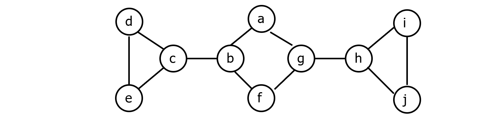
When the search is complete, if all vertices are reachable from the start vertex, a spanning tree called the depth-first search spanning tree is constructed whose edges are those inspected in the forward direction, i.e., when exploring unvisited vertices.
As a result of the traversal, the edges of an undirected graph G are classified into the following two types:
Tree edges: edges in the depth-first search tree.
Back edges: all other edges.
Input: An undirected graph G=(V, E);
Output: Preordering of the vertices in the corresponding depth-first search tree.1
2
3
4
5
6
7
8
9
10
11
12
13
14 predfn←0;
for each vertex v∈V
Mark v unvisited;
end for;
for each vertex v∈V
if v is marked unvisited then dfs(v);
end for;
dfs(v)
Mark v visited;
predfn←predfn+1;
for each edge (v, w)∈E
if w is marked unvisited then dfs(w);
end for;
Breadth-First Search(BFS)
When we visit a vertex v, we next visit all vertices adjacent to v.
This method of traversal can be implemented by a queue to store unexamined vertices.
Finding Articulation Points in a Graph
A vertex v in an undirected graph G with more than two vertices is called an articulation point if there exist two vertices u and w different from v such that any path between u and w must pass through v.
If G is connected, the removal of v and its incident edges will result in a disconnected subgraph of G.
A graph is called biconnected if it is connected and has no articulation points.
To find the set of articulation points, we perform a depth-first search traversal on G.
During the traversal, we maintain two labels with each vertex $v\in V: \alpha[v] \ and\ \beta[v]$.
$\alpha[v]$ is simply predfn in the depth-first search algorithm. $\beta[v]$ is initialized to $\alpha[v]$, but may change later on during the traversal.
For each vertex v visited, we let $\beta[v]$ be the minimum of the following:
$\alpha[v]$
$\alpha[u]$ for each vertex u such that (v, u) is a back edge
$\beta[w]$ for each vertex w such that (v, w) is a tree edge
Thus, $\beta[v]$ is the smallest $\alpha$ that v can reach through back edges or tree edges.
The articulation points are determined as follows:
The root is an articulation point if and only if it has two or more children in the depth-first search tree.
A vertex v other than the root is an articulation point if and only if v has a child w with $\beta[w]\geq \alpha[v]$.
Input: A connected undirected graph G=(V, E);
Output: Array A[1…count] containing the articulation points of G, if any.1
2
3
4
5
6Let s be the start vertex;
for each vertex v∈V
Mark v unvisited;
end for;
predfn←0; count←0; rootdegree←0;
dfs(s);1
2
3
4
5
6
7
8
9
10
11
12
13
14
15
16
17
18
19
20
21dfs(v)
Mark v visited; artpoint←false; predfn←predfn+1;
α[v]←predfn; β[v]←predfn;
for each edge (v, w) ∈ E
if (v, w) is a tree edge then
dfs(w);
if v=s then
rootdegree ← rootdegree+1;
if rootdegree=2 then artpoint←true;
else
β[v]←min{β[v], β[w]};
if β[w]>=α[v] then artpoint←true;
end if;
else if (v, w) is a back edge then β[v]←min{β[v], α[w]};
else do nothing; //w is the parent of v
end if;
end for;
if artpoint then
count←count +1;
A[count]←v;
end if;
Example: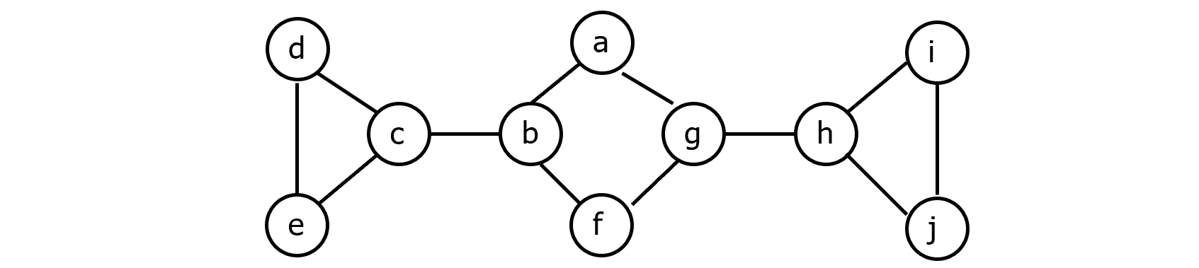
回溯 Backtracking
suitable for those problems that exhibit good average time complexity. This methodology is based on a methodic examination of the implicit state space induced by the problem instance under study. In the process of exploring the state space of the instance, some pruning takes place.
In many real world problems, a solution can be obtained by exhaustively searching through a large but finite number of possibilities. Hence, the need arose for developing systematic techniques of searching, with the hope of cutting down the search space to possibly a much smaller space.
Here, we present a general technique for organizing the search known as backtracking. This algorithm design technique can be described as an organized exhaustive search which often avoids searching all possibilities.
涂色问题 3-Color Problem
Given an undirected graph G=(V, E), it is required to color each vertex in V with one of three colors, say 1, 2, and 3, such that no two adjacent vertices have the same color. We call such a coloring legal; otherwise, if two adjacent vertices have the same color, it is illegal.
A coloring can be represented by an n-tuple (c1, c2, …, cn) such that ci∈{1, 2, 3}, $1\leq i\leq n$.
For example, (1, 2, 2, 3, 1) denotes a coloring of a graph with five vertices.
There are $3^n$ possible colorings (legal and illegal) to color a graph with n vertices.
The set of all possible colorings can be represented by a complete ternary tree called the search tree. In this tree, each path from the root to a leaf node represents one coloring assignment.
An incomplete coloring of a graph is partial if no two adjacent colored vertices have the same color.
Backtracking works by generating the underlying tree one node at a time.
If the path from the root to the current node corresponds to a legal coloring, the process is terminated (unless more than one coloring is desired).
If the length of this path is less than n and the corresponding coloring is partial, then one child of the current node is generated and is marked as the current node.
If, on the other hand, the corresponding path is not partial, then the current node is marked as a dead node and a new node corresponding to another color is generated.
If, however, all three colors have been tried with no success, the search backtracks to the parent node whose color is changed, and so on.
Example: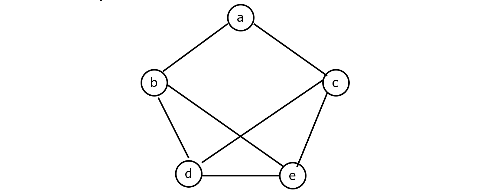
There are two important observations to be noted, which generalize to all backtracking algorithms:
(1) The nodes are generated in a depth-first-search manner.
(2) There is no need to store the whole search tree; we only need to store the path from the root to the current active node. In fact, no physical nodes are generated at all; the whole tree is implicit. We only need to keep track of the color assignment.
Recursive Algorithm
Input: An undirected graph G=(V, E).
Output: A 3-coloring c[1…n] of the vertices of G, where each c[j] is 1, 2, or 3.1
2
3
4
5
6
7
8
9
10
11
12
13
14 for k←1 to n
c[k]←0;
end for;
flag←false;
graphcolor(1);
if flag then output c;
else output “no solution”;
graphcolor(k)
for color=1 to 3
c[k]←color;
if c is a legal coloring then set flag ←true and exit;
else if c is partial then graphcolor(k+1);
end for;
Iterative Algorithm
Input: An undirected graph G=(V, E).
Output: A 3-coloring c[1…n] of the vertices of G, where each c[j] is 1, 2, or 3.1
2
3
4
5
6
7
8
9
10
11
12
13
14
15
16for k←1 to n
c[k]←0;
end for;
flag←false;
k←1;
while k>=1
while c[k]<=2
c[k]←c[k]+1;
if c is a legal coloring then set flag←true and exit from the two while loops;
else if c is partial then k←k+1;
end while;
c[k]←0;
k←k-1;
end while;
if flag then output c;
else output “no solution”;
八皇后 8-Queens Problem
How can we arrange 8 queens on an 8x8 chessboard so that no two queens can attack each other?
Two queens can attack each other if they are in the same row, column or diagonal.
The n-queens problem is defined similarly, where in this case we have n queens and an nxn chessboard for an arbitrary value of $n\geq 1$.
Consider a chessboard of size 4x4. Since no two queens can be put in the same row, each queen is in a different row. Since there are four positions in each row, there are $4^4$ possible configurations.
Each possible configuration can be described by a vector with four components x=(x1, x2, x3, x4).
For example, the vector (2, 3, 4, 1) corresponds to a configuration.
Input: none;
Output: A vector x[1…4] corresponding to the solution of the 4-queens problem.1
2
3
4
5
6
7
8
9
10
11
12
13
14
15
16for k←1 to 4
x[k]←0;
end for;
flag←false;
k←1;
while k>=1
while x[k]<=3
x[k]←x[k]+1;
if x is a legal placement then set flag←true and exit from the two while loops;
else if x is partial then k←k+1;
end while;
x[k]←0;
k←k-1;
end while;
if flag then output x;
else output “no solution”;
The General Backtracking Method
The general backtracking algorithm can be described as a systematic search method that can be applied to a class of search problems whose solution consists of a vector (x1, x2, … xi) satisfying some predefined constraints. Here, i is dependent on the problem formulation. In 3-Coloring and the 8-queens problems, i was fixed.
In some problems, i may vary from one solution to another.
Consider a variant of the PARTITION problem defined as follows. Given a set of n integers X={x1, x2, …, xn} and an integer y, find a subset Y of X whose sum is equal to y.
For instance if X={10, 20, 30, 40, 50, 60}, and y=60, then there are three solutions of different lengths: {10, 20, 30}, {20, 40}, and {60}.
Actually, this problem can be formulated in another way so that the solution is a boolean vector of length n in the obvious way. The above three solutions may be expressed by the boolean vectors {1, 1, 1, 0, 0, 0}, {0, 1, 0, 1, 0, 0}, and {0, 0, 0, 0, 0, 1}.
In backtracking, each xi in the solution vector belongs to a finite linearly ordered set Xi. Thus, the backtracking algorithm considers the elements of the cartesian product $X_1\times X_2\times…X_n$ in lexicographic order.
Initially, the algorithm starts with the empty vector. It then chooses the least element of X1 as x1. If (x1) is a partial solution, then algorithm proceeds by choosing the least element of X2 as x2. If (x1, x2) is a partial solution, then the least element of X3 is included; otherwise x2 is set to the next element in X2.
In general, suppose that the algorithm has detected the partial solution (x1, x2, …, xj). It then considers the vector v=(x1, x2, …, xj, xj+1). We have the following cases:
- If v represents a final solution to the problem, the algorithm records it as a solution and either terminates in case only one solution is desired or continues to find other solutions.
- If v represents a partial solution, the algorithm advances by choosing the least element in the set Xj+2.
- If v is neither a final nor a partial solution, we have two subcases:
- If there are still more elements to choose from in the set Xj+1, the algorithm sets xj+1 to the next member of Xj+1.
- If there are no more elements to choose from in the set Xj+1, the algorithm backtracks by setting xj to the next member of Xj. If again there are no more elements to choose from in the set Xj, the algorithm backtracks by setting xj-1 to the next member of Xj-1, and so on.
分枝界限 Branch and Bound (TSPs)
Branch and bound design technique is similar to backtracking in the sense that it generates a search tree and looks for one or more solutions.
However, while backtracking searches for a solution or a set of solutions that satisfy certain properties (including maximization or minimization), branch-and-bound algorithms are typically concerned with only maximization or minimization of a given function.
Moreover, in branch-and-bound algorithms, a bound is calculated at each node x on the possible value of any solution given by nodes that may later be generated in the subtree rooted at x. If the bound calculated is worse than the previous bound, the subtree rooted at x is blocked.
Henceforth, we will assume that the algorithm is to minimize a given cost function; the case of maximization is similar. In order for branch and bound to be applicable, the cost function must satisfy the following property.
For all partial solutions (x1, x2, …, xk-1) and their extensions (x1, x2, …, xk), we must have
Given this property, a partial solution (x1, x2, …, xk) can be discarded once it is generated if its cost is greater than or equal to a previously computed solution.
Thus, if the algorithm finds a solution whose cost is c, and there is a partial solution whose cost is at least c, no more extensions of this partial solution are generated.
Traveling Salesman Problems (TSPs):
Given a set of cities and a cost function that is defined on each pair of cities, find a tour of minimum cost. Here a tour is a closed path that visits each city exactly once. The cost function may be the distance, travel time, air fare, etc.
An instance of the TSP is given by its cost matrix whose entries are assumed to be nonnegative.
With each partial solution (x1, x2, …, xk), we associate a lower bound y, which is the cost of any complete tour that visits the cities x1, x2, …, xk in this order must be at least y.
Observations:
We observe that each complete tour must contain exactly one edge and its associated cost from each row and each column of the cost matrix.
We also observe that if a constant r is subtracted from every entry in any row or column of the cost matrix A, the cost of any tour under the new matrix is exactly r less than the cost of the same tour under A. This motivates the idea of reducing the cost matrix so that each row or column contains at least one entry that is equal to 0. We will refer to such a matrix as the reduction of the original matrix.
Let (r1, r2, …, rn) and (c1, c2, …, cn) be the amounts subtracted from rows 1 to n and columns 1 to n, respectively, in an nxn cost matrix A. Then, y defined as follow is a lower bound on the cost of any complete tour.
随机 Randomized Algorithms
Based on the probabilistic notion of accuracy.
One form of algorithm design in which we relax the condition that an algorithm must solve the problem correctly for all possible inputs, and demand that its possible incorrectness is something that can safely be ignored due to its very low likelihood of occurrence.
Also, we will not demand that the output of an algorithm must be the same in every run on a particular input.
A randomized algorithm can be defined as one that receives, in addition to its input, a stream of random bits that it can use in the course of its action for the purpose of making random choices.
A randomized algorithm may give different results when applied to the same input in different rounds. It follows that the execution time of a randomized algorithm may vary from one run to another when applied to the same input.
Randomized algorithms can be classified into two categories:
The first category is referred to as Las Vegas algorithms. It constitutes those randomized algorithms that always give a correct answer, or do not give an answer at all.
The second category is referred to as Monte Carlo algorithms. It always gives an answer, but may occasionally produce an answer that is incorrect. However, the probability of producing an incorrect answer can be make arbitrarily small by running the algorithm repeatedly with independent random choices in each run.
Randomized Selection
Input: An array A[1…n] of n elements and an integer k, $1\leq k\leq n$;
Output: The kth smallest element in A;
1.rselect(A, 1, n, k);1
2
3
4
5
6
7
8
9
10rselect(A, low, high, k)
v←random(low, high);
x←A[v];
Partition A[low…high] into three arrays:
A1={a|a<x}, A2={a|a=x}, A3={a|a>x};
case
|A1|>=k: return select (A1, 1, |A1|, k);
|A1|+|A2|>=k: return x;
|A1|+|A2|<k: return select(A3, 1, |A3|, k-|A1|-|A2|);
end case;
Testing String Equality
Suppose that two parties A and B can communicate over a communication channel, which we will assume to be very reliable. A has a very long string x and B has a very long string y, and they want to determine whether x=y.
Obviously, A can send x to B, who in turn can immediately test whether x=y. But this method would be extremely expensive, in view of the cost of using the channel.
Another alternative would be for A to derive from x a much shorter string that could serve as a “fingerprint” of x and send it to B.
B then would use the same derivation to obtain a fingerprint for y, and then compare the two fingerprints.
If they are equal, then B would assume that x=y; otherwise he would conclude that $x\ne y$. B than notifies A of the outcome of the test.
This method requires that transmission of a much shorter string across the channel.
For a string w, let I(w) be the integer represented by the bit string w. One method of fingerprinting is to choose a prime number p and then use the fingerprint function
If p is not too large, then the fingerprint Ip(x) can be sent as a short string. If $I_p(x)\ne I_p(y)$, then obviously $x\ne y$. However, the converse is not true. That is, if Ip(x)=Ip(y), then it is not necessarily the case that x=y. We refer to this phenomenon as a false match.
In general, a false match occurs if $x\ne y$, but $I_p(x)=I_p(y)$, i.e., p divides $I(x)-I(y)$.
The weakness of this method is that, for fixed p, there are certain pairs of strings x and y on which the method will always fail. Then, what’s the probability?
Let n be the number of bits of the binary strings of x and y, and p be a prime number which is smaller than $2n^2$. The probability of false matching is 1/n.
Thus, we choose p at random every time the equality of two strings is to be checked, rather than agreeing on p in advance. Moreover, choosing p at random allows for resending another fingerprint, and thus increasing the confidence in the case x=y.
- A chooses p at random from the set of primes less than M.
- A sends p and Ip(x) to B.
- B checks whether Ip(x)=Ip(y) and confirms the equality or inequality of the two strings x and y.
Pattern Matching
Given a string of text $X=x_1x_2…x_n$ and a pattern $Y=y_1y_2…y_m$, where $m\leq n$, determine whether or not the pattern appears in the text. Without loss of generality, we will assume that the text alphabet is $\sum=\{0, 1\}.$
The most straightforward method for solving this problem is simply to move the pattern across the entire text, and in every position compare the pattern with the portion of the text of length m.
This brute-force method leads to an $O(mn)$ running time in the worst case.
Here we will present a simple and efficient Monte Carlo algorithm that achieves a running time of $O(n+m)$.
The algorithm follows the same brute-force algorithm of sliding the pattern Y across the text X, but instead of comparing the pattern with each block $X(j)=x_jx_{j+1}…x_{j+m-1}$, we will compare the fingerprint $I_p(Y)$ of the pattern with the fingerprints $I_p(X(j))$ of the blocks of text.
The key observations that when we shift from one block of text to the text, the fingerprint of the new block X(j+1) can easily be computed from the fingerprint of X(j).
If we let $W_p=2^m$ (mod p), then we have the recurrence
Input: A string of text X and a pattern Y of length n and m, respectively.
Output: The first position of Y in X if Y occurs in X; otherwise 0.1
2
3
4
5
6
7
8
9Choose p at random from the set of primes less than M;
j←1;
Compute Wp=2^m (mod p), Ip(Y) and Ip(Xj);
while j<=n-m+1
if Ip(Xj)=Ip(Y) then return j ; \\A match is found (probably)
Compute Ip(Xj) using previous equation;
j←j+1;
end while;
return 0; //Y does not occur in X (definitely)
The time complexity of the previous pattern matching algorithm is O(m+n).
Let p be a prime number which is smaller than 2mn2. The probability of false matching is 1/n.
To convert the algorithm into a Las Vegas algorithm is easy.
Whenever the two fingerprints Ip(Y) and Ip(X(j)) match, the two strings are tested for equality.
Thus, we end with an efficient pattern matching algorithm that always gives the correct result, and the time complexity is still O(m+n).
逼近 Approximation Algorithms
Compromise on the quality of solution in return for faster solutions.
There are many hard combinatorial optimization problems that cannot be solved efficiently using backtracking or randomization.
An alternative in this case for tacking some of these problems is to devise an approximation algorithm, given that we will be content with a “reasonable” solution that approximates an optimal solution.
Associated with each approximation algorithm, there is a performance bound that guarantees that the solution to a given instance will not be far away from the neighborhood of the exact solution.
A marking characteristic of (most of) approximation algorithms is that they are fast, as they are mostly greedy algorithm.
A combinatorial optimization problem $\Pi$ is either a minimization problem or a maximization problem. It consists of three components:
(1) A set $D_\Pi$ of instances.
(2) For each instance $I\in D_\Pi$, there is a finite set $S_\Pi(I)$ of candidate solutions for I.
(3) Associated with each solution $\sigma\in S_\Pi(I)$ to an instance I in $D_\Pi$, there is a value $f_\Pi(\sigma)$ called the solution value for $\sigma$.
If $\Pi$ is a minimization problem, then an optimal solution $\sigma’$ for an instance $I\in D_\Pi$ has the property that for all $\sigma\in S_\Pi(I)$, $f_\Pi(\sigma’)\leq f_\Pi(\sigma)$. An optimal solution for a maximization problem is defined similarly. We will denote by OPT(I) the value $f_\Pi(\sigma)$.
An *approximation algorithm A for an optimization problem $\Pi$ is a (polynomial time) algorithm such that given an instance $I\in D_\Pi$, it outputs some solution $\sigma\in S_\Pi(I)$. We will denote by $A(I)$ the value $f_\Pi(\sigma)$.
Difference Bounds
The most we can hope from an approximation algorithm is that the difference between the value of the optimal solution and the value of the solution obtained by the approximation algorithm is always constant.
In other words, for all instances I of the problem, the most desirable solution that can be obtained by an approximation algorithm A is such that $|A(I)-OPT(I)|\leq K$, for some constant K.
Planar Graph Coloring
Let G=(V, E) be a planar graph. By the Four Color Theorem, every planar graph is four-colorable. It is fairly easy to determine whether a graph is 2-colorable or not. On the other hand, to determine whether it is 3-colorable is NP-complete.
Given an instance I of G, an approximation algorithm A may proceed as follows:
Assume G is nontrivial, i.e. it has at least one edge. Determine if the graph is 2-colorable. If it is, then output 2; otherwise output 4. If G is 2-colorable, then $|A(I)-OPT(I)|=0$. If it is not 2-colorable, then $|A(I)-OPT(I)\leq 1$. This is because in the latter case, G is either 3-colorable or 4-colorable.
Counterexample: Knapsack Problems
There is no approximation algorithms with difference bounds for knapsack problems.
Relative Performance Bounds
Clearly, a difference bound is the best bound guaranteed by an approximation algorithm.
However, it turns out that very few hard problems possess such a bound. So we will discuss another performance guarantee, namely the relative performance guarantee.
Let $\Pi$ be a minimization problem and I an instance of $\Pi$. Let A be an approximation algorithm to solve $\Pi$. We define the approximation ratio $R_A(I)$ to be
If $\Pi$ is a maximization problem, then we define $R_A(I)$ to be
Thus the approximation ratio is always greater than or equal to one.
The Bin Packing Problem
Given a collection of items u1, u2, …, un of sizes s1, s2, …, sn, where such sj is between 0 and 1, we are required to pack these items into the minimum number of bins of unit capacity.
We list here one heuristic method:
First Fit (FF): The bins are indexed as 1, 2, … All bins are initially empty. The items are considered for packing in the order u1, u2, …, un. To pack item ui, find the least index j such that bin j contains at most 1-si, and add item ui to the items packed in bin j. Then, we have
网络流 Network Flow
A network is a 4-tuple (G, s, t, c), where G=(V, E) is a directed graph, s and t are two distinguished vertices called, respectively, the source and sink, and c(u, v) is a capacity function defined on all pairs of vertices with c(u, v)>0 if (u, v) ∈ E and c(u, v)=0 otherwise. |V|=n, |E|=m.
A flow in G is a real-valued function f on vertex pairs having the following four conditions:
(1) Skew symmetry. $\forall u, v\in V, f(u, v)=-f(v, u)$. We say there is a flow from u to v if $f(u, v)>0$.
(2) Capacity constraints. $\forall u, v\in V, f(u, v)\leq c(u, v)$. We say edge (u, v) is saturated if $f(u, v)=c(u, v)$.
(3) Flow conservation. $\forall u\in V-\{s, t\}, \sum_{v\in V}f(u, v)=0$. In other words, the net flow (total flow out minus total flow in) at any interior vertex is 0.
(4) $\forall v\in V, f(v, v)=0$.
A cut {S, T} is a partition of the vertex set V into two subsets S and T such that $s\in S$ and $t\in T$. The capacity of the cut {S, T}, denoted by c(S, T), is
The flow across the cut {S, T}, denoted by f(S, T), is
Thus, the flow across the cut {S, T} is the sum of the positive flow on edges from S to T minus the sum of the positive flow on edges from T to S.
For any vertex u and any subset $A\subseteq V$, let f(u, A) denote f({u}, A), and f(A, u) denote f(A, {u}). For a capacity function c, c(u, A) and c(A, u) are defined similar.
The value of a flow f, denoted by |f|, is defined to be
Lemma: For any cut {S, T} and a flow f, |f|=f(S, T).
Max-Flow Problems: Design a function f for the network (G, s, t, c), so that |f| is the maximum.
Given a flow f on G with capacity function c, the residual capacity function for f on the set of pairs of vertices is defined as follows.
For each pair of vertices, $u, v\subseteq V$, the residual capacity $r(u, v)=c(u, v)-f(u, v)$. The residual graph for the flow f is the directed graph $R=(V, E_f)$, with capacities defined by r and
The residual capacity r(u, v) represents the amount of additional flow that can be pushed along the edge (u, v) without violating the capacity constraints.
If $f(u, v)<c(u, v)$, then both (u, v) and (v, u) are present in R. If there is no edge between u and v in G, then neither (u, v) nor (v, u) are in $E_f$. Thus, $|E_f|\leq 2|E|$.
Example: what’s the residual graph of the following graph?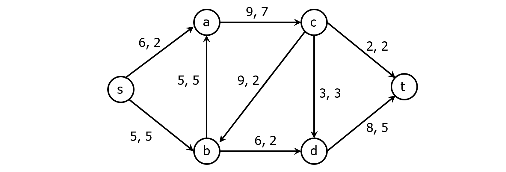
Let f and f’ be any two flows in a network G. Define the function f+f’ by (f+f’)(u, v)=f(u, v)+f’(u, v) for all pairs of vertices u and v. Similarly, define the function f-f’ by (f-f’)(u, v)=f(u, v)-f’(u, v).
Lemma: Let f be a flow in G and f’ the flow in the residual graph R for f. Then the function f+f’ is a flow in G of value |f|+|f’|.
Lemma: Let f be any flow in G and f* a maximum flow in G. If R is the residual graph for f, then the value of a maximum flow in R is |f*|-|f|.
Given a flow f in G, an augmenting path p is a directed path from s to t in the residual graph R. The bottleneck capacity of p is the minimum residual capacity along p. The number of edges in p will be denoted by |p|.
Theorem (max-flow min-cut theorem): Let (G, s, t, c) be a network and f a flow in G. The following three statements are equivalent:
(a) There is a cut {S, T} with c(S, T)=|f|.
(b) f is a maximum flow in G.
(c) There is no augmenting path for f.
The Ford-Fulkerson Method:
The previous theorem suggests a way to construct a maximum flow by iterative improvement
One keeps finding an augmenting path arbitrarily and increases the flow by its bottleneck capacity
Input: A network (G, s, t, c);
Output: A flow in G;1
2
3
4
5
6
7
8
9
10
11Initialize the residual graph: R←G;
for each edge (u, v)∈E
f(u, v)←0;
end for;
while there is an augmenting path p=s, …, t in R
Let ▲ be the bottleneck capacity of p;
for each edge (u, v) in p
f(u, v) ←f(u, v)+ ▲;
end for;
Update the residual graph R;
end while;
The time complexity of the Ford-Fulkerson Method is O(m|f*|), where m is the number of edges and |f*| is the value of the maximum flow, which is an integer.
Shortest Path Augmentation:
Here we consider another heuristic that puts some order on the selection of augmenting paths.
Definition: The level of a vertex v, denoted by level(v), is the least number of edges in a path from s to v. Given a directed graph G=(V, E), the level graph L is (V’, E’), where V’ is the set of vertices can be reached from s and
Given a directed graph G and a source vertex s, its level graph L can easily be constructed using breadth-first search.
MPLA | Minimum path length augmentation
Minimum path length augmentation (MPLA)
MPLA selects an augmenting path of minimum length and increases the current flow by an amount equal to the bottleneck capacity of the path. The algorithm starts by initializing the flow to the zero flow and setting the residual graph R to the original network. It then proceeds in phases. Each phase consists of the following two steps:
(1) Compute the level graph L from the residual graph R. If t is not in L, then halt; otherwise continue.
(2) As long as there is a path p from s to t in L, augment the current flow by p, remove saturated edges from L and R and update them accordingly.
Input: A network (G, s, t, c);
Output: The maximum flow in G;1
2
3
4
5
6
7
8
9
10
11
12
13
14for each edge (u, v)∈ E
f(u, v)←0;
end for;
Initialize the residual graph: R ← G;
Find the level graph L of R;
while t is a vertex in L
while t is reachable from s in L
Let p be a path from s to t in L;
Let ▲ be the bottleneck capacity on p;
Augment the current flow f by ▲;
Update L and R along the path p;
end while;
Use the residual graph R to compute a new level graph L;
end while;
匹配 Matching
Given an undirected graph G=(V, E), |V|=n, and |E|=m. A matching in G is a subset $M\subseteq E$ such that no two edges in M have a vertex in common.
An edge $e\in E$ is matched if it is in M, and unmatched or free otherwise.
A vertex $v\in E$ is matched if it is incident to a matched edge, and unmatched or free otherwise.
The size of a matching M, i.e. the number of matching edges in it, will be denoted by |M|.
A maximum matching in a graph is a matching of maximum cardinality. A perfect matching is one in which every vertex in V is matched.
The maximum matching problem asks for a subset $M\subseteq E$ with the maximum number of nonoverlapping edges; that is, no two edges in M have a vertex in common.
This problem arises in many applications, particularly in the areas of communication and scheduling.
Given a matching M in an undirected graph G=(V, E), an alternating path p with respect to M is a simple path that consists of alternating matched and unmatched edges. The length of p is denoted by |p|.
If the two endpoints of an alternating path coincide, then it is called an alternating cycle.
An alternating path with respect to M is called an augmenting path with respect to M if all the matched edges in p are in M and its endpoints are free.
Let M1 and M2 be two matchings in a graph G. Then
That is, $M1\oplus M2$ is the set of edges that are in M1 or in M2 but not in both.
Lemma: Let M be a matching and p an augmenting path with respect to M, then $M\oplus p$ is a matching of size $|M\oplus p|=|M|+1$.
Corollary: A matching M in an undirected graph G is maximum if and only if G contains no augmenting paths with respect to M.
Theorem: Let M1 and M2 be two matchings in an undirected G such that |M1|=r, |M2|=s and s>r. Then, $M1\oplus M2$ contains at least k=s-r vertex-disjoint augmenting paths with respect to M1.
二分图的匈牙利树方法 Hungarian Tree Method for Bipartite Graphs
The previous Lemma and Corollary suggest a procedure for finding a maximum matching in G:
Starting from an arbitrary (e.g. empty) matching, we find an augmenting path p in G, invert the roles of the edges in p (matched to unmatched and vice-versa), and repeat the process until there are no more augmenting paths.
However, to find an augmenting path efficiently in a general graph is not easy.
Given an undirected graph G=(V, E), if V can be divided into two disjoint subsets X and Y so that each edge in E has an end in X and an end in Y, then G is a bipartite graph.
The most important feature of a bipartite graph is it contains no cycles of odd length.
Finding an augmenting path in the case of bipartite graphs is much easier than in the case of general graphs.
Let $G=(X\cup Y, E)$ be a bipartite graph with |X|+|Y|=n and |E|=m. Let M be a matching in G. We call a vertex in X an x-vertex. Similarly, a y-vertex denotes a vertex in Y.
First, we pick a free x-vertex, say r, and label it outer. From r, we grow an alternating path tree, i.e., a tree in which each path from the root r to a leaf is an alternating path. This tree, call it T, is constructed as follows:
Starting from r, add each unmatched edge (r, y) connecting r to the y-vertex y and label y inner.
For each y-vertex y adjacent to r, add the matched edge (y, z) to T if such a matched edge exists, and label z outer.
Repeat the above procedure and extend the tree until either a free y-vertex is encountered or the tree is blocked, i.e., cannot be extended any more (note that no vertex is added to the tree more than once).
If a free y-vertex is found, say v, then the alternating path from the root r to v is an augmenting path. On the other hand, if the tree is blocked, then in this case the tree is called a Hungarian tree.
Next, we start from another free x-vertex, if any, and repeat the above procedure.
Observation
If T is a Hungarian tree, then it cannot be extended; each alternating path traced from the root is stopped at some outer vertex.
The only free vertex in T is its root. Notice that if (x, y) is an edge such that x is in T and y is not in T, then x must be labeled inner. Otherwise, x must be connected to a free vertex or T is extendable through x.
It follows that no vertex in a Hungarian tree can occur in an augmenting path.
Suppose that p is an alternating path that shares at least one vertex with T. If p “enters” T, then it must be through a vertex labeled inner. If it “leaves” T, then it must also be through a vertex labeled as inner. But, then, p is not an alternating path; a contradiction.
Therefore, if, in the process of searching for an augmenting path, a Hungarian tree is found, then it can be removed permanently without affecting the search.
Input: A bipartite graph $G=(X\cup Y, E)$;
Output: A maximum matching M in G;1
2
3
4
5
6
7
8Initialize M to any arbitrary (possibly empty) matching;
while (there exists a free x-vertex and a free y vertex)
Let r be a free x-vertex, and using breadth-first
search, grow an alternating path tree T rooted at r;
if (T is a Hungarian tree) then let G←G-T;
else (find an augmenting path p in T and let
M=M $\oplus$ p);
end while.