基于图的图像分割

Graph-Based Segmentation 是经典的图像分割算法。论文：Efficient Graph-Based Image Segmentation，IJCV 2004，MIT，作者 Pedro F. Felzenszwalb.

图

图是由顶点集$V$（vertices）和边集$E$（edges）组成，表示为$G=(V,E)$，顶点$v \in V$，在本文中即为单个的像素点，连接一对顶点的边$(v_i,v_j)\in E$具有权重$w(v_i,v_j)$，本文中的意义为顶点之间的不相似度，所用的是无向图。

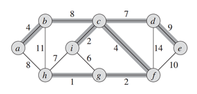树：特殊的图，图中任意两个顶点，都有路径相连接，但是没有回路。如上图中加粗的边所连接而成的图。如果看成一团乱连的珠子，只保留树中的珠子和连线，那么随便选个珠子，都能把这棵树中所有的珠子都提起来。如果，i和h这条边也保留下来，那么顶点h,i,c,f,g就构成了一个回路。

最小生成树（MST, minimum spanning tree）：特殊的树，给定需要连接的顶点，选择边权之和最小的树。上图即是一棵MST
本文中，初始化时每一个像素点都是一个顶点，然后逐渐合并得到一个区域，确切地说是连接这个区域中的像素点的一个MST。如图，棕色圆圈为顶点，线段为边，合并棕色顶点所生成的MST，对应的就是一个分割区域。分割后的结果其实就是森林。

相似性

既然是聚类算法，那应该依据何种规则判定何时该合二为一，何时该继续划清界限呢？
对于孤立的两个像素点，所不同的是颜色，自然就用颜色的距离来衡量两点的相似性，本文中是使用RGB的距离，即

$$\sqrt{(r_1-r_2)^2+(g_1-g_2)^2+(b_1-b_2)^2}$$

当然也可以用perceptually uniform的Luv或者Lab色彩空间，对于灰度图像就只能使用亮度值了，此外，还可以先使用纹理特征滤波，再计算距离，比如，先做Census Transform再计算Hamming distance距离。

自适应阈值

上面提到应该用亮度值之差来衡量两个像素点之间的差异性。对于两个区域（子图）或者一个区域和一个像素点的相似性，最简单的方法即只考虑连接二者的边的不相似度。

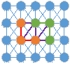已经形成了棕色和绿色两个区域，现在通过紫色边来判断这两个区域是否合并。那么我们就可以设定一个阈值，当两个像素之间的差异（即不相似度）小于该值时，合二为一。迭代合并，最终就会合并成一个个区域，效果类似于区域生长.

显然，对上面这张图如果设置全局阈值并不合适，那么自然就得用自适应阈值。对于p区该阈值要特别小，s区稍大，h区巨大。

In this section we define a predicate, D, for evaluating whether or not there is evidence for a boundary between two components in a segmentation (two regions of an image).This predicate is based on measuring the dissimilarity between elements along the boundary of the two components relative to a measure of the dissimilarity among neighboring elements within each of the two components. The resulting predicate compares the inter-component differences to the within component differences and is thereby adaptive with respect to the local characteristics of the data.
We define the internal difference of a component C ⊆ V to be the largest weight in the minimum spanning tree of the component, MST(C, E). That is,

$$Int(C)=\max\limits_{e\in MST(C,E)}w(e)$$

One intuition underlying this measure is that a given component C only remains connected when edges of weight at least Int(C) are considered.
We define the difference between two components C1, C2 ⊆ V to be the minimum weight edge connecting the two components. That is,

$$Diff(C_1,C_2)=\min\limits_{v_i\in C_1,v_j\in C_2,(v_i,v_j)\in E}w((v_i,v_j))$$

If there is no edge connecting C1 and C2 we let Dif(C1, C2) = ∞. This measure of difference could in principle be problematic, because it reflects only the smallest edge weight between two components. In practice we have found that the measure works quite well in spite of this apparent limitation. Moreover, changing the definition to use the median weight, or some other quantile, in order to make it more robust to outliers, makes the problem of finding a good segmentation NP-hard, as discussed in the Appendix. Thus a small change to the segmentation criterion vastly changes the difficulty of the problem.

The region comparison predicate evaluates if there is evidence for a boundary between a pair or components by checking if the difference between the components, Dif(C1, C2), is large relative to the internal difference within at least one of the components, Int(C1) and Int(C2). A threshold function is used to control the degree to which the difference between components must be larger than minimum internal difference. We define the pairwise comparison predicate as,

$$D(C_1,C_2)= \begin{equation} \left\{ \begin{array}{lr} true，diff(C_1,C_2)>MInt(C_1,C_2) \\ flase，otherwise \end{array} \right. \end{equation}$$

where the minimum internal difference, MInt, is defined as,

$$MInt(C_1,C_2)=min(Int(C_1)+\tau(C_1),Int(C_2)+\tau(C_2))$$

The threshold function τ controls the degree to which the difference between two components must be greater than their internal differences in order for there to be evidence of a boundary between them (D to be true). For small components, Int(C) is not a good estimate of the local characteristics of the data. In the extreme case, when |C| = 1, Int(C) = 0. Therefore, we use a threshold function based on the size of the component,

$$\tau (C)=k/|C|$$

where |C| denotes the size of C, and k is some constant parameter. That is, for small components we require stronger evidence for a boundary. In practice k sets a scale of observation, in that a larger k causes a preference for larger components. Note, however, that k is not a minimum component size. Smaller components are allowed when there is a sufficiently large difference between neighboring components.

Any non-negative function of a single component can be used for τ without changing the algorithmic results in Section 4. For instance, it is possible to have the segmentation method prefer components of certain shapes, by defining a τ which is large for components that do not fit some desired shape and small for ones that do. This would cause the segmentation algorithm to aggressively merge components that are not of the desired shape. Such a shape preference could be as weak as preferring components that are not long and thin (e.g., using a ratio of perimeter to area) or as strong as preferring components that match a particular shape model. Note that the result of this would not solely be components of the desired shape, however for any two neighboring components one of them would be of the desired shape.

算法步骤

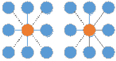
Step 1: 计算每一个像素点与其8邻域或4邻域的不相似度。

Step 2: 将边按照不相似度non-decreasing排列（从小到大）排序得到$e_1,e_2,……,e_N$。
Step 3: 选择$e_1$
Step 4: 对当前选择的边$e_n$进行合并判断。设其所连接的顶点为$(v_i,v_j)$。如果满足合并条件：

1. $v_i,v_j$不属于同一个区域$Id(V_i)\ne Id(v_j)$
2. 不相似度不大于二者内部的不相似度。$w_{i,j}\leq Mint(C_i,C_j)$则执行Step 5，否则执行Step 6。

Step 5: 更新阈值以及类标号。
更新类标号：将$Id(v_i),Id(v_j)$的类标号统一为$Id(v_i)$的标号。
更新该类的不相似度阈值为：$w_{i,j}+\frac{k}{|c_i|+|c_j|}$。
注意：由于不相似度小的边先合并，所以，$w_{i,j}$即为当前合并后的区域的最大的边，即$Int(C_i\cup C_j)=w_{i,j}$。
Step 6: 如果$n\leq N$，则按照排好的顺序，选择下一条边转到Step 4，否则结束。

参考

https://blog.csdn.net/ttransposition/article/details/38024557